EXTENT OF THE CORONA
Glenn Schneider, University of Arizona
Jay Pasachoff & Steve Souza, Williams College
CALIBRATION NOTES
Subsequent to the initialweb posting regarding these data, the individual 40ms integration CCDframes taken on the flight deck gyro platform of QF 2901 with an SBIG ST2000XMCCD, have been instrumentally calibrated. Each of the frames hadsubtracted from them a dark/bias reference frame (made from a median combinationof 25 dark/bias frames taken on the aircraft just prior to the eclipseimaging sequence), and were fat fielded as well (see Post Processing fora note on flat fielding). A wide-field image mosaic created from the calibratedoffset pointed frames (as previously discussed) and is shown here in severalforms.
NOTE: ALL images on or linked from this page are produced at 1/4 theoriginal pixilization to facilitate web-based display. The originalCCD matrix BEFORE enlarging the image composite by combining offset pointedfields (see above) was 1600x1200 pixels. Any discussion related to"pixels" here is in the 1/4-size (1/16 array) resampled pixel space unlessotherwise noted.
IMAGE DEPTH and RADIAL EXTENT
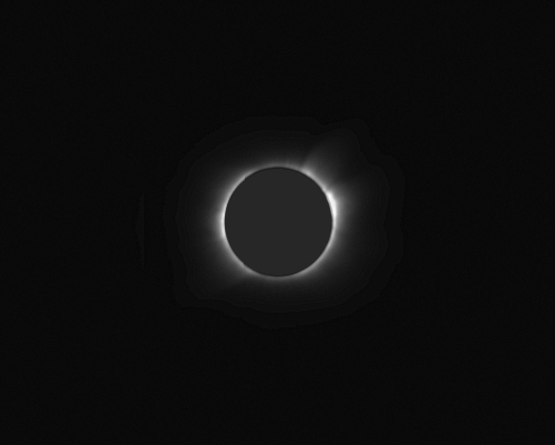
How deep did we go? This is illustrated in a linear display ofthe final wide-field mosaic in a linear display stretch to show the fullradial extent of the corona. In this hard stretch at the bottom ofthe dynamic range, little information is conveyed about the structure withinthe corona.
EXTENT OF THE CORONA
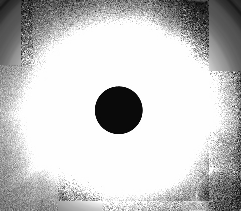
We imaged the corona to a distance of at least 6 Solar radii from theheliocenter (see the radial profile below). Indeed, at an even harderstretch than shown above, one can still see declining isophotes at theedge of the mosaiced field. At such a hard stretch the Moon appears. At this extreme level of displayed surface brightness the limb of the Moonwould be diffused by scattered light. As a visualization aid, theinset dark circle is a mask which is 2% larger than the apparent (mean)lunar angular diameter. During the imaging sequence, from which thisimage mosaic/composite was made, the Moon was moving across the sun, sothis mask fully contains its displaced position with respect to the Sunover that time. In instrumental units, this image is displayed ata stretch from 0 to 100 counts, where the median surface brightness ofthe inner corona immediately adjacent to the occulted photosphere was measuredat 100,000 counts.
LINEAR DISPLAYS
It is impossible to capture the full extent of the dynamic range ofthe solar corona recorded on the QF2901 flight deck CCD imager in a singlelinear image display image display. Indeed about 10 are needed giventhe appx. 1/4% stepped intensity display depths (per channel) on most computermonitors. Indeed, about 10 images are needed, as shown in the QuickTimemovie, prepared earlier with the data still in uncalibrated form.
DISPLAY TRANSFORMATIONS & RADIAL SURFACE BRIGHTNESS("GRADIENT") FILTERING
An effective way to collapse the dynamic display range is to performa non-linear numerical transformation on the data. In doing so, however,as the image contrast in any given radial zone (which declines outwardfrom the Sun) is also collapsed. Hence, in any given radial zonethe structural features in the corona are not as apparent as in a lineardisplay specifically optimized in display stretch for the surface brightnessof that zone. To mitigate this (to various degrees) one can subtractthe underlying radial brightness profile of the corona before displayingthe image, which then improves the image contrast for features such ascoronal streamers, holes, etc. Most image editing programs, suchas Photoshop, provide "features" for "radial gradient" masking. However,one cannot specify the quantitative form of the radial mask, and if notproperly matched to the data themselves, zonal artifacts are introduces. Additionally, but subjectively, radial gradient masking is often done withtoo heavy a hand, which results in a coronal with very star image contrastsin its internal features, which for esthetics (rather than photometric)purposes is often displeasing.
A proper radial gradient filter should be made from the data themselves. I do this by computing the median radial surface brightness profile, in1 pixel wide annular zones, and then very modestly smoothing the profile(with a 2 pixel boxcar) to reduce the effect of any anomalously brightor dark zones due to uncompensated pixel defects. In the case ofthe above image, here is the radial surface brightness profile, expressedas a median per-pixel intensity with respect to a median pixel the brightestcircum-solar zone in a log (base 10) plot:
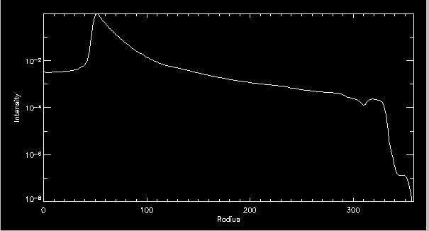
CORONAL SURFACE BRIGHTNESS PROFILE (self-normalized)
As you can see we imaged the corona very well (at high S/N) out to adistance of 300 (1/4 size resampled) image pixels. The angular radiusof the Sun is appx. 45 image pixels (hence agreeing with the earlier statement"we imaged the corona to a distance of at least 6 Solar radii from theheliocenter". The sharp drop-off beyond the R ~ 300 pixel regionis where the data become both photon starved and field size constrained.
In subtracting a MEDIAN radial profile one must take care not to locallyoversubtract. With this data set subtracting more than 30% of theprofile intensity begins to "dig holes" in the image where it is brightest- in the inner corona adjacent to the lunar limb (you can see the risingpower in the surface brightness profile at small radii near the limb). Being very conservative, so that no negative residuals arise at any radialzones, images were produces subtracting 20% of the profile. Theseare shown, first, in square root displays.
SQUARE ROOT DISPLAYS
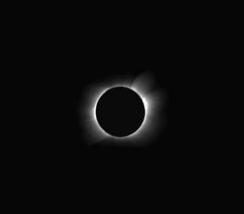
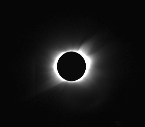
Displaying the square root of the data, after 20% radial profile subtraction,allow showing most of the coronal dynamic range in only three images asillustrated below:
 |
 |
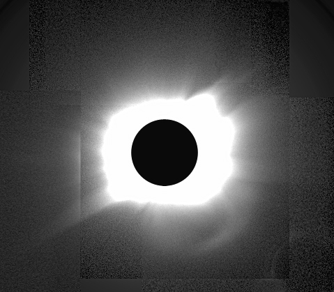 |
Note the extent and structure of the coronal streamers beyond the region,in each display, beyond where the display is saturated. The verticaland horizontal lines are artifacts of imperfect flat-fielding in combiningthe image data taken with different field pointings. The flat-fieldillumination source used to ascertain the inter-pixel CCD response maynot have been intrinsically uniform (see Flat Field discussion), whichmakes photometric calibration at the lowest signal levels difficult (ifnot impossible). The brighter diffuse arc, are below the sun andto right at about 3 solar radii from the heliocenter, is an artifact dueto an afocal image ghost, likely from a multiple reflection off the aircraftwindow.
LOGARITHMIC DISPLAYS
To further collapse the radial dynamic range in the image display alogarithmic transformation can be applied. (Here I use log base 10, whichmakes it easy to keep track of transformed intensities, but any logarithmicbase can be used as desired). Such a display will result in a slightlycontrast in specific radial zones, but does indeed show the global structureof the coronal at a glance.
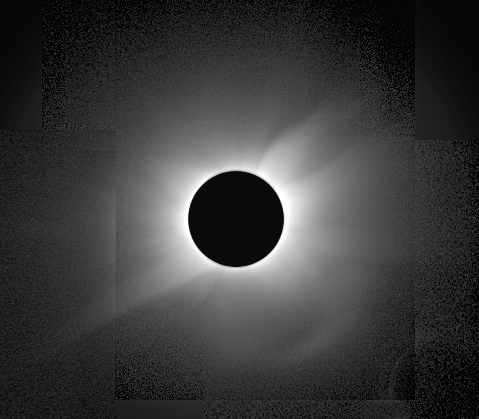
LOGARITHMIC DISPLAY
To he image above is displayed over [3.8] dex after subtracting 20%of the radial brightness profile - a dynamic range of appx 6,300. Contrasts "improvements" can be had at the expense of saturating he displayin the center, clipping the extent of the corona at large radii, or introducinga small level of negative residuals by a modest oversubtraction of theradial surface brightness profile.
CONTRAST ENHANCEMENT
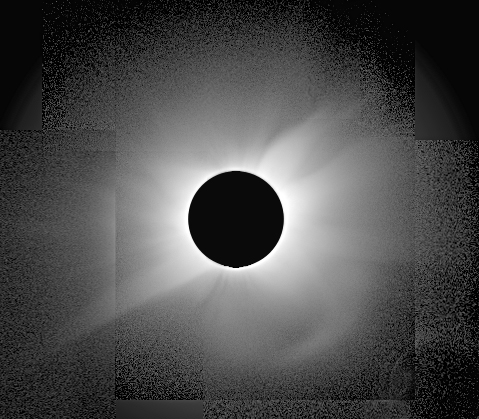
Moderate contrast improvement over most of the radial range, at theexpense of the introduction of some quantization noise at large distance,may be had by taking the product of the above two transformations, anddisplaying the product itself in a logarithmic stretch. For thesedata, first subtraction a 30% profile is warranted (and supported by thedata) as it results in only a very small local region of oversubtraction- which sharp eyed observers will see as a few "extra" dark pixels in thefollowing image just at the bottom of the 2% oversized lunar mask:
FLAT-FIELD ERRORS, IMAGE MOSAICS, and SPATIALFILTERING
The above image mosaic is not "seamless". This is primarily aresult of residual photometric errors in the attempted flat-field compensation.The flat field calibration frames (from which a calibration reference filewas made and applied to the individual eclipse images) were obtained priorto shipment of the equipment to Australia/Antarctica by Steve Souza (WilliamsCollege). While these frames taken with the optical system (lensand filter) in place and exposed on a uniformly illuminated target,these were not sky flats, and hence not at infinity. Examinationof the flatted image data obtained from the eclipse, at different fieldpointings, indicates residual large-scale (global) flat-field errors. Theseare likely due to focus-dependent vignetting in the optical system, pointing-dependentdiffuse stray light scattered/reflected from the aircraft window, or acombination of both. Empirical corrections to the differential flat-fielderrors were assessed from the image-overlap areas in the ensemble of offset-pointedtarget frames. These corrections were then applied to the image mosaicwhich, for the most part, removed the differential flat-field errors. These errors, before correction, are most severe on frame boundaries bothbecause of detector edge defects, and very different S/N across over-lapboundaries because of the small number of frames. Corrections torows and columns along the boundaries themselves, works best by assessingthe needed corrections after performing a mild gradient-edge enhancementto the images. This process (subtracting a fraction of the localmedian about every pixel) is similar to "unsharp masking". When properlycontrolled this process also spatially filters the image to bring out higherspatial frequency information in the corona, but at the modest expenseof accentuating the pixel-to-pixel noise in the low S/N regions of theimage. The result, with some subjectivity in tuning parameters, isshown below, and except for some further subjectivity in how to presentthe data (contrast, spatial filter bandwidth, dynamic range clipping, etc.)this is very likely about the "best" which can be obtained from these data(and, it makes a pretty nice picture!):
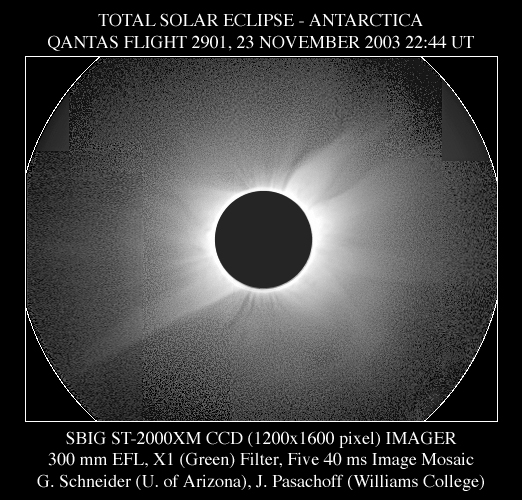
"Final"* Wide-Feild Mosaic Image of TSE 2003 fromQF 2901
* it's never really final, of course...
Two notes:
1) This above flat-field error compensation process worked very wellin an intra-field and inter-frame sense (as the image above demonstrates). Bringing frame 11_04 (lower left) under control was much more difficult,and uncompensated systematic can still be seen - though at a very low level.
2) The surface brightness excess in the region of the previously notedafocal image ghost (at 3 R(sun) to the lower right) was assessed in comparisonto the median surface brightness at the same radial zones, excluding thiscontaminated sector. This excess was then "removed" (by intensityscaled subtraction) from each pixel whose intensity exceeded by 3-sigmathe azimuthal median at the same radius. The intensity subtractedwas the fraction of the intensity at that point in 3-sigma excess. This, too, is imperfect, but is a marked improvement.
NOTE: ALL images here are produced at 1/4 the original pixilizationto facilitate web-based display. The original CCD matrix BEFORE enlargingthe image composite by combining offset pointed fields (see above) was1600x1200 pixels. Any discussion related to "pixels" here is in the1/4-size (1/16 array) resampled pixel space unless otherwise noted.
SOHO/LASCO L2, QF 2901 & SOHO/EIT
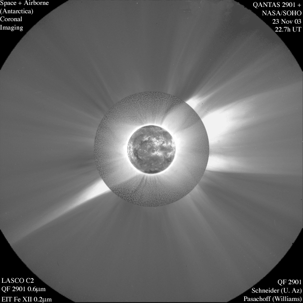
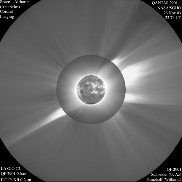
The LASCO (Large Angle Spectrometric coronagraph) L2 Coronagraph, andthe EIT (Extreme-Ultraviolet Imaging Telescope) on NASA'sSOHO spacecraft were imaging the solar coronal and photosphere, respectively,at times very close (and during) the eclipse. Our QF 2901 FlightDeck imager, during totality, covered an inner radial region which cannotbe reached by this space-based facility. An image composite of outercorona with SOHO/LASCO L2, mid and inner corona from QF 2901, and the photospherewith SOHO/EIT, all nearly contemporaneous, is shown below.
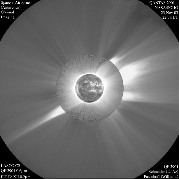
QF 2901 (Airborne) + SOHO (Space) Imaging of TSE 2003
(Alternate representations: QF2901 clipped, QF 2901 smoothed)
The LASCO C2 image was prepared (by the SOHO project) independentlyfrom the QF 2901 image, and was provided in non-quantitative form (as aJPEG file) with its brightest regions hard-stretched to white, and witha linearity transfer which differs from the QF 2901 processed image. Hence, the "boundary" between the two images appears somewhat discontinuousin local intensity and in their radial brightness gradients, but is presentedin this form to illustrate the morphology of the coronal structures fromthe photosphere outward. With the actual LASCO C2 data, which weare requesting, we should be able to re-present this equitably for bothdata sets. In addition, because there is a region of overlap in theLASCO C2 and QF 2901 imagery, we should be able to cross-calibrate thetwo data sets and obtain an absolute radiometric calibration (subject tofilter band transfer uncertainties) of the entire corona. Stay tuned.
Return to Glenn Schneider'sHome Page